Benchmark Problems for Acoustical Parameters
Column 1:
Relationship between background noise and reverberation time
Introduction
Reverberation time can be calculated from the slope of the energy decay curve (Schroeder curve) computed by the backward integration of a squared impulse response signal. However, there is a case that the energy decay curve does not have a linear slope. We can think of several possible reasons for that such as the room is not diffuse or the background noise being too high masking the decay part of the reverberation. In this column, a method described in Section 5.3.3 of ISO 3382-1:2009 to reduce the effect of background noise is introduced regarding the latter issue.Background Noise is a Cause of Reverberation Time Calculation Error
Impulse response in the benchmark problem B11 is an artificial response (shown in Figure 1) made to have 1.5 seconds of reverberation time with whitenoise added to simulate background noise. Reverberation time is computed for each of the octave bands. As an example, let us take a look at 500 Hz band of the response. Figure 2 shows the impulse response for an octave band centered at 500 Hz. Figure 3 shows the energy decay curve of the same benchmark problem of which the blue curve showing the decay curve, green curve showing the curve within the regression range, and red line showing the linear regression fit to it.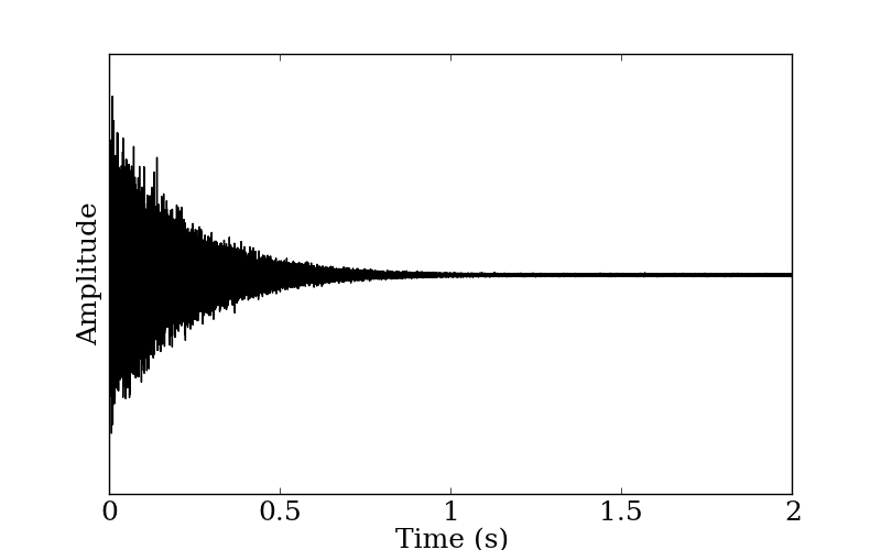
Figure 1: Impulse response of the benchmark problem B11.
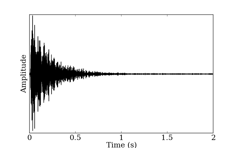
Figure 2: Impulse response of the benchmark problem B11 (for an octave band centered at 500 Hz).
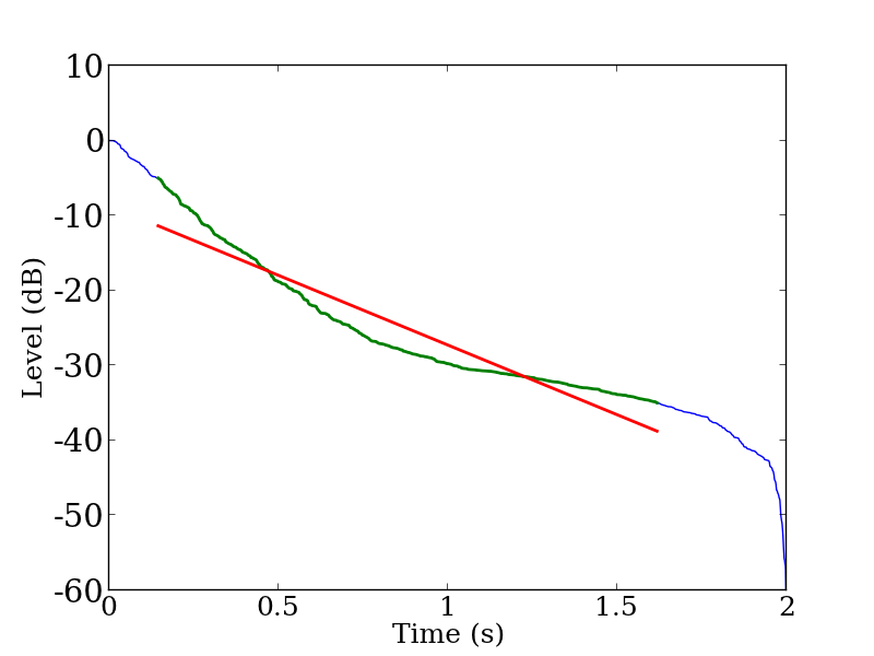
Figure 3: Decay curve of the benchmark problem B11 (for an octave band centered at 500 Hz).Blue curve denote the energy decay curve, green curve denote the curve within the regression range, and red line denote the linear fit.
As we can see from the Figure 3, the slope of the decay curve is becoming less steep before it reaches the lower bound of T30 regression range (–35 dB). The cause of this curvature is the background noise. The linear regression line (red line in the figure) does not fit well with the decay part of the curve and thus is not sufficient for reading reverberation time from the curve.
Checking the signal-to-noise ratio
According to ISO3382-1, it is suggested to have more than 45 dB of signal peak level to background noise level ratio (SNR hereafter) in order to calculate T30. This implies that the effect of the background noise is negligible if the level of the background noise is more than 10 dB lower than the signal at near –35 dB of the regression line.We can check whether the SNR is sufficient by reading the energy decay of the impulse response by plotting the squared values of the response. For example, squared impulse response of 500 Hz band is shown as black lines in Figure 4. It can be seen from the curve at around –35 dB that SNR is approximately 40 dB, and effect of such low SNR has to be taken into account. There are ways to overcome the low SNR, such as using narrower regression ranges used in T20 or compensating the effect of background noise in the reverberation time calculation. However, these countermeasures are ad-hoc and do not work against many cases with very high background noise.
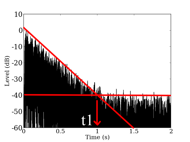
Figure 4: Squared impulse response of the benchmark problem B11 (1-octave band at 500 Hz, black lines) and two regression lines (red) to calculate t1.
Using Different Level Range for Regression
The decay curve in Figure 3 is almost linear from 0 dB down to –25 dB. The result of linear regression on the interval between –5 dB and –25 dB is shown in Figure 5. Because the linear part of the decay curve is regressed adequately it is expected to that the correct reverberation time can be calculated using T20. Note that limiting the regression range will reduce the number of points to be used for the regression computation and a small amount of variance in the values will affect the slope of the regression line. Result of T20 is shown in Figure 7. Discussion is given later with the compensation method explained next.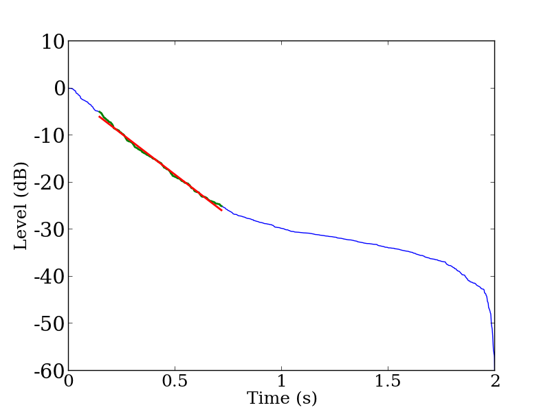
Figure 5: Decay curve of the benchmark problem B11 (500 Hz band). Blue curve denote the decay curve, green curve denote the curve within the regression range, and red line denote the linear fit.
Background Noise Compensation
The problem we face is due to the integration of background noise energy at the late part of the impulse response. The following method can be used to compensate for the background noise to achieve adequate reverberation time calculation.First, we compute t1 which indicates the time that the energies of impulse response signal and background noise are approximately equal. t1 is the time at the intersection of horizontal line fit to the background noise level and the linear regression line on the decay part of the squared signal of band-pass filtered impulse response signal (Figure 4).
Compensated energy decay curve is calculated with the following equation,
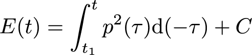 (1)
(1)where C is the constant value to compensate for the background noise after t1. The correct reverberation time can be achieved when C is calculated as squared sum of energy assuming that the impulse response energy decays linearly after t1. Details of C computation are stated in Section 5.3.3 of ISO3382-1 and in the reference [1]. Energy decay curve after the compensation is shown in Figure 6.
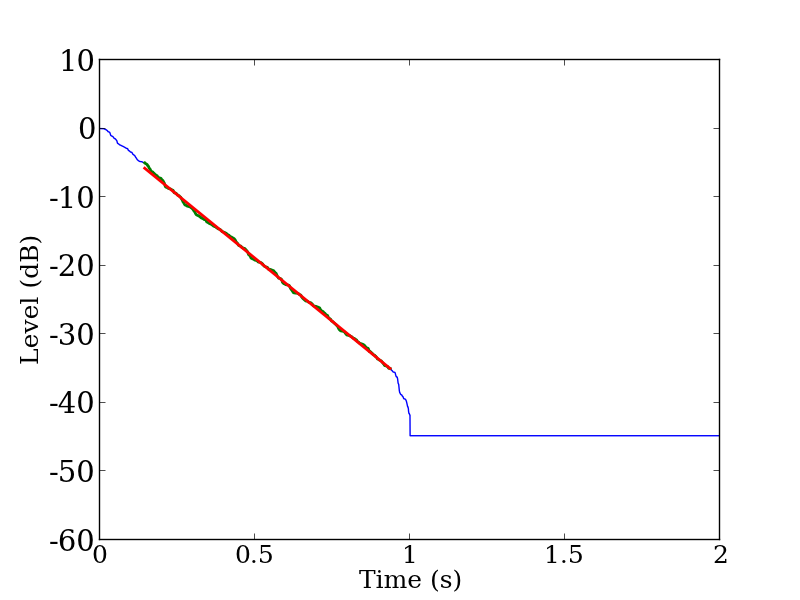
Figure 6: Energy decay curve calculated with equation 1 (500 Hz band). Blue curve denote the decay curve, green curve denote the curve within the regression range, and red line denote the linear fit.
From Figure 6, the decay curve is linear at the regression range of –5 dB to –35 dB and reverberation time (T30) can be adequately read from the graph. T30 without the background noise compensation (hence integrated over all duration of the response), T30 with the compensation (hence backward integration starting from t1), and T20 which uses the regression range of –5 dB and –25 dB are shown in Figure 7.
Figure 7: Reverberation time for each octave band. (Black lines show T30 calculated from the decay curve without background compensation, red lines show T30 calculated with background noise compensation, and blue lines show T20.)
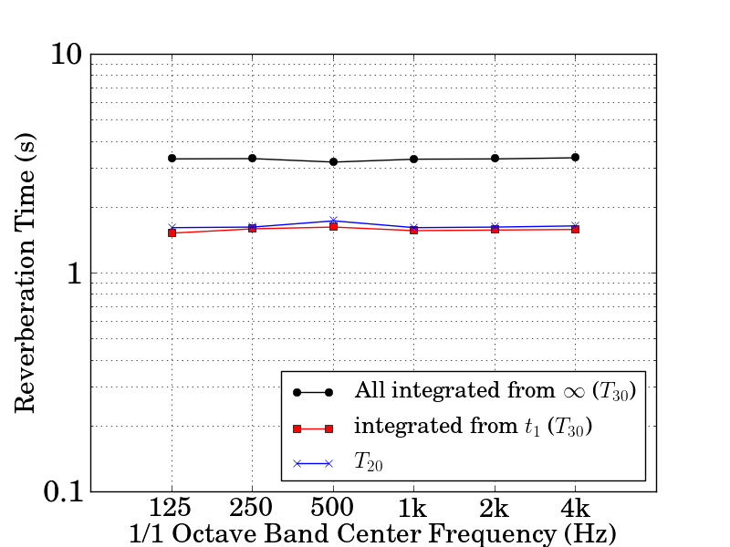
Figure 7: Reverberation time for each octave band. (Black lines show T30 calculated from the decay curve without background compensation, red lines show T30 calculated with background noise compensation, and blue lines show T20.)
As can be seen in Figure 7, there are more than two fold differences between T30 without compensation (about 3.2 seconds) and T30 with compensation (1.5 seconds). Not fitting the regression line adequately on to the linear part of the curve results in mistakes in reading reverberation time.In addition, curvature in energy decay curve due to background noise is affected by the ratio of the energy of signal before t1 and the energy of background noise after t1. That is, although the adequate SNR is examined by looking at the plot of squared impulse response, there is a caveat that there may be a curvature from the beginning of the decay curve when duration of the background noise part is very long.
Countermeasures
The following countermeasures should be used for calculation of the correct reverberation time:- draw a squared response for each octave-band filtered signal, and check that the background noise is at least 10 dB lower than the lower bound of the regression range (e.g., –35 dB for T30),
- draw an energy decay curve for each octave-band filtered signal using t1 described above,
- draw an energy decay curve and a linear regression line for each octave-band filtered signal and check if the regression line fits to the linear part of the decay curve, and
- if the above two do not improve the T30 computation calculate the reverberation time with different regression range such as T20.