Benchmark Problems for Acoustical Parameters
Column 2:
Reading correct reverberation time from insufficient decay length
Introduction
Reverberation time can be calculated from the slope of the energy decay curve (Schroeder curve) computed by the backward integration of a squared impulse response signal. However, there are cases that sufficient duration of the decay curve for reading reverberation time was not obtained due to impulse response signal being too short. This problem often occurs in spaces with long reverberation such as atrium, gymnasium, and large exhibition spaces. In this column, how to estimate the reverberation time from such an impulse response is introduced.Effect of data length of an impulse response on reading the reverberation time
Impulse response of the benchmark problem B12 was created from the problem A13. The benchmark problem A13 is 6.0 seconds long signal made from applying 3.0 seconds of exponential decay to whitenoise. The first 1.65 seconds was extracted from problem A13 to create the problem B12, hence it has reverberation time of 3.0 seconds while the data length is only 1.65 seconds. The impulse response of the problem B12 is shown in Figure 1, squared impulse response of 1000 Hz band is shown in Figure 2, and the energy decay curve of 1000 Hz band is shown in Figure 3.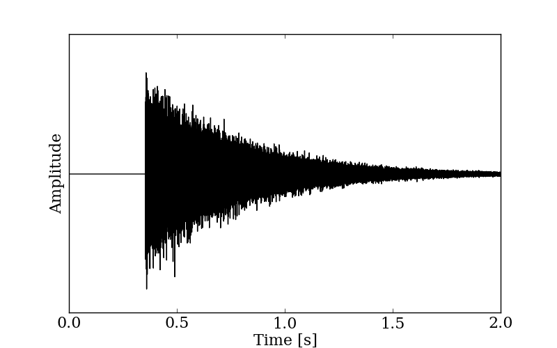
Figure 1: Impulse response of the benchmark problem B12.
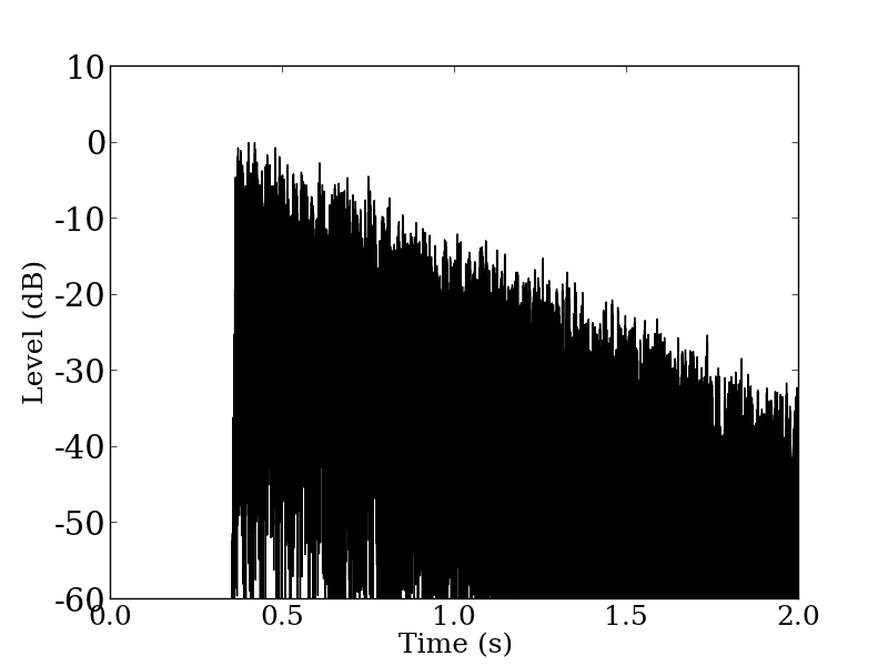
Figure 2: Squared impulse response of the benchmark problem B12 (1000 Hz band).
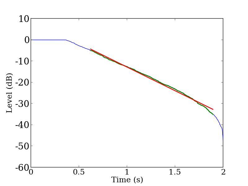
Figure 3: The energy decay curve of the benchmark problem B12 (1000 Hz band). Blue curve denote the energy decay curve, green curve denote the curve within the regression range, and red line denote the linear fit.
ISO3382-1 states that the level of the signal has to be at least 45 dB higher than the level of background noise in order to calculate T30. The signal shown in Figure 2 does not have enough energy to calculate T30, because the decay of the signal has not reached the background noise level and 45 dB signal-to-noise ratio necessary to read T30 is not available. The end part of the energy decay curve in Figure 3 decreases rapidly since the integration range becomes shorter along the time axis. Hence, the curve’s convex curvature is seen before the curve reaches the lower bound of T30 calculation which is –35 dB.When calculating T30, regression on this energy decay curve will include the convex part as shown in Figure 3 resulting in shorter reverberation time than the actual time. One way around this problem is to use different regression range so that the regression line is fit to the linear part of the energy decay curve.
Using different regression range
We now know that it is difficult to estimate the reverberation time from T30 for the impulse response in the benchmark problem B12. Now we can try to estimate the reverberation time by changing the lower bound of the regression range. The squared impulse response shown in Figure 2 only decays down to about –35 dB, hence we will consider setting the lower bound to –25 dB and computing T20 using the data between –5 dB and –25 dB. Figure 4 shows the result of the regression analysis on the energy decay curve for 1000 Hz band.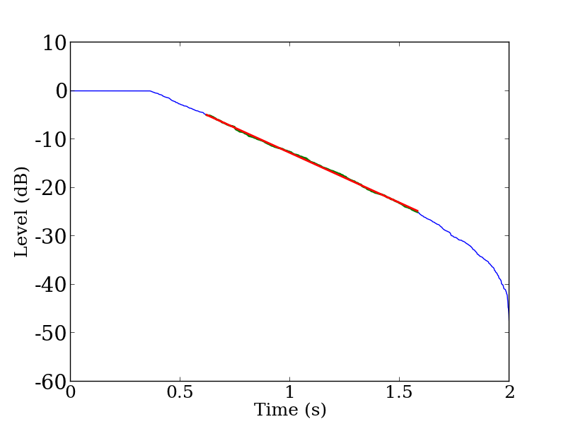
Figure 4: Energy decay curve shown in Figure 1 (1000 Hz band) with different regression range. Blue curve denote the decay curve, green curve denote the curve within the regression range (from –5 dB to –25 dB), and red line denote the linear fit.
Since sufficient fit was achieved on the linear part of the decay curve, the reading of the reverberation time is expected to be adequately correct. Since the impulse response of the benchmark problem B12 had only about 35 dB of decay in all frequency bands from 125 Hz to 4 000 Hz, T20 was calculated with the regression range from –5 dB to –25 dB for all bands.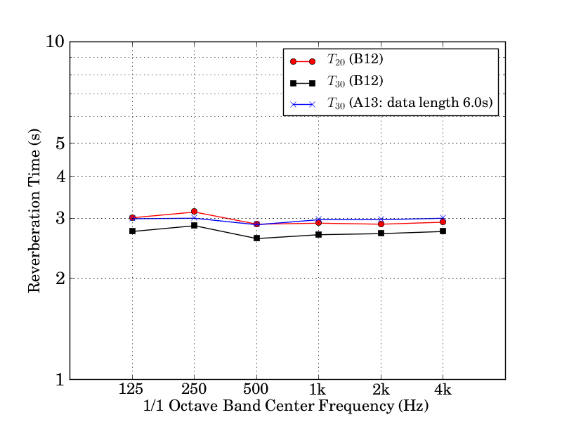
Figure 5: Reverberation times for octave bands.
The impulse response in the problem A13 and B12 are the same, and ideally the same reverberation time is computed. Seeing T30 calculated from the problem A13 (blue lines) as a target, T30 calculated from B12 (black lines) is 0.3 seconds shorter at maximum. Also, although T20 calculated from B12 (red lines) is 0.1 seconds difference at maximum, the value is closer to the target than that of T30. Therefore, T20 was a better index of the reverberation time for this particular problem of B12.
In order to estimate the reverberation time from impulse responses with insufficient decay time such as the one seen in the problem B12, changing the regression range is desirable. However, decreasing the interval to too short range will allow little variations in the values affect its linear fit. The range has to be taken as wide as possible.
Relation of duration of decay part and reverberation time
When measuring an impulse response, the data length has to be decided according to the rough estimate of the reverberation time. The question is how do we decide the necessary duration of the measurement.Reverberation time is defined as the time for the room energy density to get reduced by 60 dB. However we use –45 dB reduction of the energy for T30, namely the time for the energy decay needs to be more than 75% of the reverberation time.
The energy decay curve was drawn for the impulse response of the problem A13, but with varying the start time of the backward integration. The start time was changed from 1.5 seconds to 4.0 seconds in 0.25 seconds interval. Figure 6 shows the impulse response of the problem A13 and Figure 7 shows the energy decay curve at 500 Hz band. The linear slope down to –35 dB can be seen in the integration time larger than 2.25 seconds. This also suggests that the length of the data has to have more than 75% of the reverberation time. Obviously, the recording time of the signal will be longer since it includes the time for the direct sound to reach the microphones.
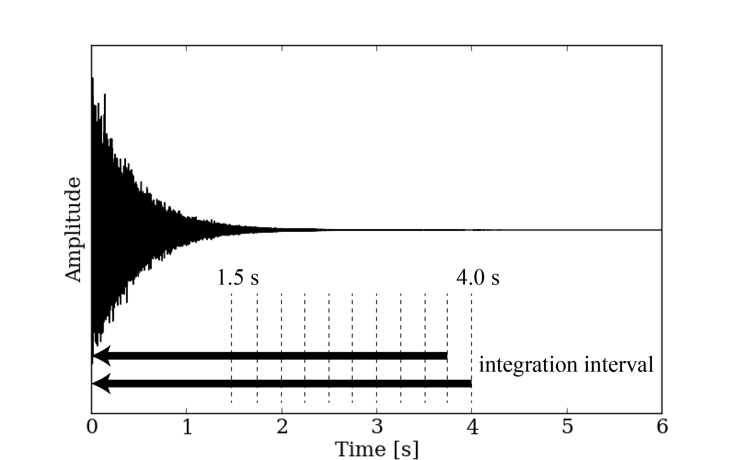
Figure 6: Impulse response of the benchmark problem A13.
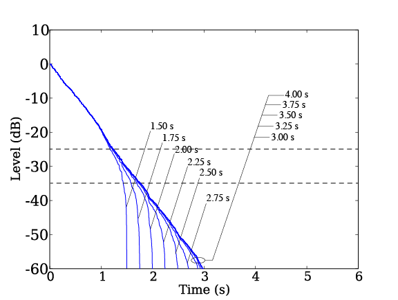
Figure 7: Energy decay curve with varying start time of the backward integration (500 Hz band).
Countermeasures
Following countermeasures are proposed for the impulse response signal with insufficient duration of measurement:- draw squared impulse response for each octave band and look for the level of the regression range with sufficient linear slope,
- regression range must be taken as wide as possible, and
- draw energy decay curve for each octave band and check that the decay curve and linear regression fits well.